This article is part 1 of a two-part series. The second part—how to analyze a staged rollout—is here.
Confidence intervals are one of the most misunderstood and misused concepts in all of statistics. I recently had a conversation about confidence intervals that bugged me greatly because A. I was only 70% sure my intuition was correct, and B. I couldn’t explain my intuition in a coherent, convincing way.
![]()
Here’s the (fictionalized) scenario: a staged rollout of a new website feature. We plan to show the new feature to 10% of our users and measure the click-through rate (CTR).1 The VP in charge says we’ll make a decision based on the worst-case scenario; we’ll launch to everybody as long as the experiment result isn’t catastrophically bad. We run the test and the point estimate from our sample is a CTR of 7.3%, with a 95% confidence interval of [6.8%, 7.8%]. Now it’s decision time; the conversation goes something like this:
(J)unior Data Scientist: Can we consider 6.8% the worst-case scenario for the true CTR?
(S)enior Data Scientist: No, I don’t think so. The confidence interval definition doesn’t let us make probabilistic statements about a parameter.
J: Right, but that’s not what I’m saying. The definition says that if we were to repeat this experiment 100 times, 95 of the runs on average would produce a confidence interval that covers the parameter. So that means that our particular interval has a 95% chance of being correct, i.e. containing the parameter. And that implies there’s only a 2.5% probability the parameter is less than 6.8%.
S: Hmm, that’s an interesting way to put it, but…my statistical spidey-sense is tingling; it doesn’t feel right. I’m afraid I can’t explain exactly why, though.
J: What does the confidence interval even mean then? What’s the point if not to give an intuition about the best and worst probable outcomes?
S: That’s a great question. Come to think of it, I’m not sure what the purpose is of a specific, realized confidence interval after the fact. Why don’t we try a Bayesian approach that will give us the interpretation we want?
J: Because I don’t know Bayesian statistics, and it feels reasonable to use the confidence interval for this purpose, and you haven’t convinced me that I’m wrong. I’m going for it.
S: Sigh…2
Our common-sense intuition about confidence intervals has a way of overwhelming the facts. As our fictional Junior Data Scientist says, what’s the point of a confidence interval, if not to give worst and best case bounds? How can it be that 95% of confidence intervals cover the true parameter, but our specific interval doesn’t have 95% probability of containing the parameter?
What does ‘worst-case scenario’ mean?
Let’s step back for a second and define what business stakeholders mean by “worst-case scenario”. In my experience, this is how decision-makers often think: > if it’s unlikely our metric is truly worse than some business-critical threshold, then > we’ll go ahead with our plan.
Formalizing this will help. The true value of our metric (e.g. CTR) is our parameter of interest, let’s call it $ $. The worst-case scenario is the event that $$ is actually less than some business-critical threshold.
\[ \theta \leq \textrm{threshold} \]
What our decision-makers want to know is the probability of this event: \[ \mathbb{P}(\theta \leq \textrm{threshold}) \]
If the probability is sufficiently low, like less than 2.5% then we roll out our feature. If not, we roll the test back and try something else.
The key data science question is: can we use a confidence interval to relate the decision threshold to the probability of the event occurring? Specifically, if we use the lower bound of the confidence interval as the decision threshold, can we bound the probability of the event? In our fictional scenario, for example, can we claim the following? \[ \mathbb{P}(\theta \leq 6.8\%) < 0.025 \]
Why can’t we use the confidence interval as a worst-case threshold?
The answer is no, but let’s first build some intuition by playing a dice game. I’m going to roll a die and look at the result without showing you; your goal is to guess what the number is (this is your parameter). I’m generous so I’ll allow you to make your guess in the form of a range, either 1 through 3 or 4 through 6. I’m also a bad liar so even though you can’t see the die itself, you can guess the right interval 95% of the time just by reading my reaction.
I roll the die and look at the result; it’s a 3. You see my reaction and guess the number is between 4 and 6. Imagine now asking what’s the probability 3 is between 4 and 6? Or saying because we guess right 95% of the time, there’s only a 5% chance that 3 is not between 4 and 6. It doesn’t make any sense at all—your specific guess either includes the correct answer or it doesn’t, even if you don’t know the correct answer. In this case, you guessed wrong and your interval does not include the correct answer. There’s nothing probabilistic about it.3
This is exactly what happens with confidence intervals. In frequentist statistics—the philosophy to which confidence intervals belong—the parameter is a fixed but unknown fact of the universe, analogous to the result of my die roll that I know but don’t show you. A 95% confidence level describes how often our intervals (i.e. guesses) are correct, but once we’ve drawn a sample and computed a specific confidence interval (i.e. made a guess), there’s nothing random about whether the parameter is inside that specific interval.
What we can say with frequentist inference is that 95% of the samples we could draw would yield a confidence interval that contains the true value of our metric. This gives us the faith to assume the specific interval we compute is correct and to act accordingly.4 In our running example, suppose our fictional VP said we would proceed with the new feature rollout if we believe the true CTR is at least 6.5%. Because our confidence interval lower bound is higher than this, we can assume the true CTR is not that low, and proceed with the rollout.
Frankly, this is pretty weak. We said in the section above we wanted the probability that the true CTR is below some decision threshold, and this approach cannot give us that. It cannot quantify the consequences if our interval happens to have come from one of the rare un-representative draws. And it can’t tell us how likely the bad-but-not-worst-case outcomes are within the confidence interval.
How does the confusion arise?
I think there are three reasons why our intuition insists we can use confidence intervals to make probabilistic conclusions about parameters.
First, the language used to describe confidence intervals is misleading. Many writers describe confidence intervals with ambiguous language like:5
We are 95% confident the parameter is contained in the interval [6.8%, 7.8%].
This language is naturally but incorrectly interpreted as a statement about degree-of-belief, along the lines of:
There is a 95% probability the parameter is inside our specific confidence interval. That means there’s only a 2.5% probability the parameter is less than the lower bound of the confidence interval.
Sadly, the term confidence in the first statement does not imply any probabilities about the parameter. It just means we typically make good guesses with our intervals.
The second source of confusion comes from the way confidence intervals are typically taught: with emphasis on the mechanics of interval construction. Introductory treatments often start with a picture of a Gaussian distribution centered on the sample statistic.6 The standard errors are counted off on both sides of the mean and the probability mass between each interval is highlighted. The conclusion is that to trap 95% of the probability, set your confidence interval to extend two standard errors on either side of the sample statistic.
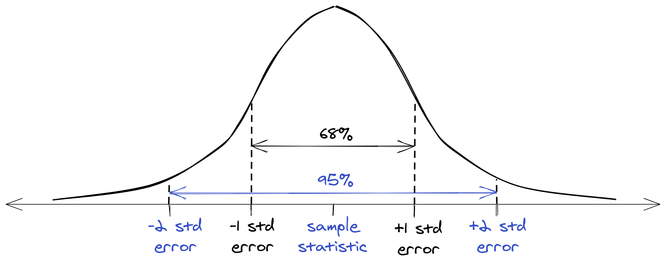
This kind of plot makes it seem like the sample statistic is the quantity that’s fixed; there’s no indication what’s actually random. The student reasonably fills in the gap by assuming the random thing is the parameter. From here, it’s obvious that a confidence interval can be interpreted as a probabilistic statement about the parameter.
In my opinion, we should start instead with the core frequentist model, which looks more like this:
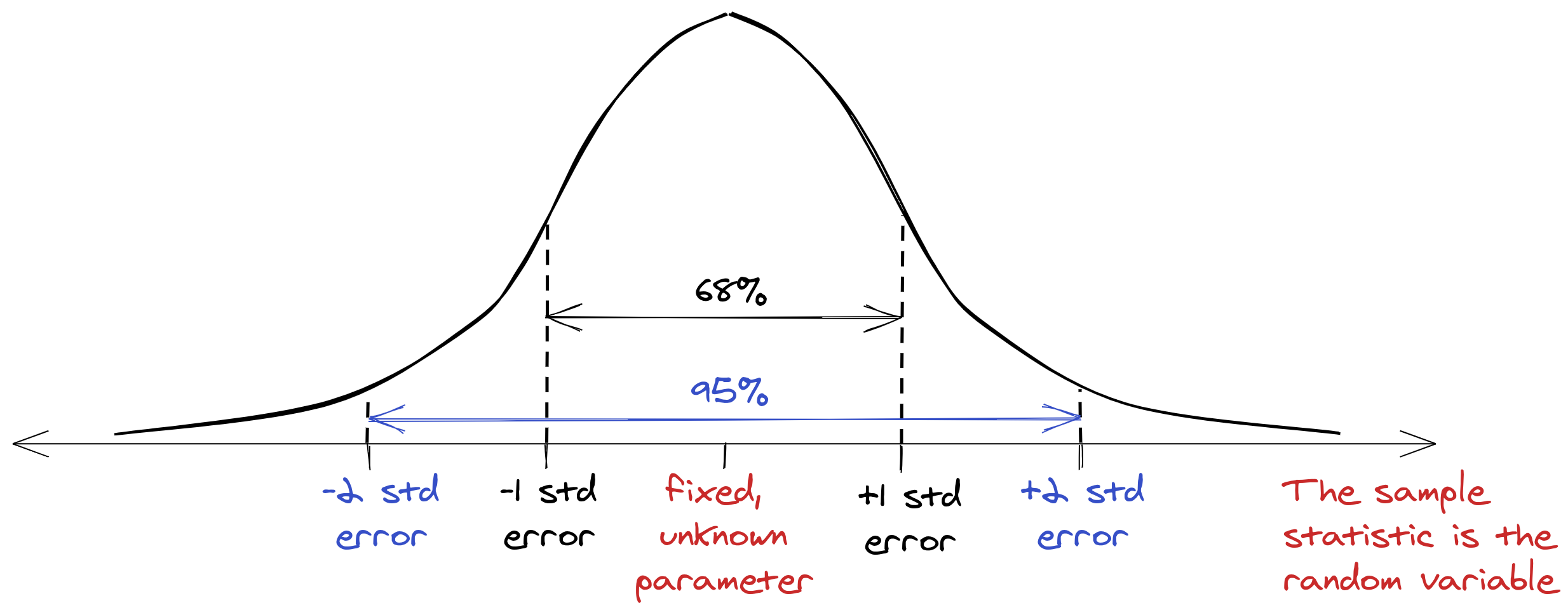
Now we can clearly see the parameter is the central anchor around which the sample statistic and confidence intervals (CI) vary, over many samples.
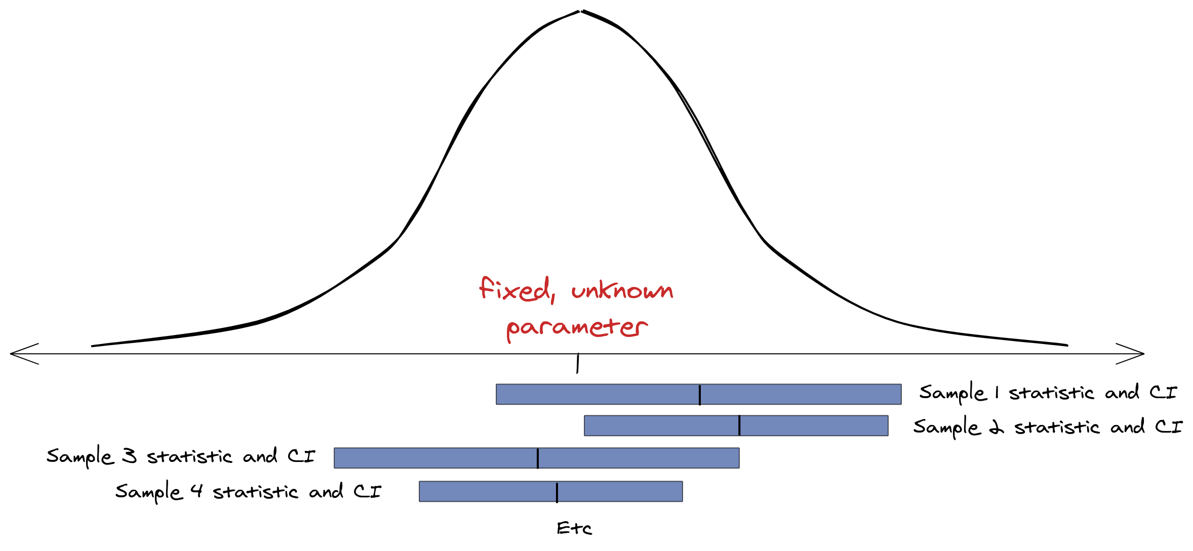
We don’t know the parameter, of course, so we have to use the sample to estimate the parameter and the standard error.7 We also typically only have a single sample, point estimate, and confidence interval, even though the coverage properties of the confidence interval refer to hypothetical repeated samples.
As the previous two figures show, most of the samples we could draw would yield confidence intervals that cover the parameter, but we can’t know whether the sample we actually observed gave us one of rare, extreme intervals that does not. We can also see from this figure that the confidence interval is not a probabilistic statement about the parameter. The solid blue bar is the interval we’ve constructed from the sample we’ve observed; there’s no way to ask what the probability is of the parameter being in the interval—it just isn’t.
Finally, the third reason our intuition insists on using confidence intervals is that’s all most of us learned in school. Without the tools to answer our original question, what else is there to do?
How do I get a worst-case estimate then?
The quantity we want to evaluate, \(\mathbb{P}(\theta \leq 6.8\%)\), is a probabilistic statement about the parameter \(\theta\) (remember, this is the unknown true value of our metric of interest).
Bayesian statistics gives us the tools we need. In Bayesian inference, parameters are random quantities, so it’s totally fine to make a probabilistic statement about them. In particular, the concept of a credible interval answers our worst-case scenario question. This is an interval that contains the parameter of interest with some specified probability, based on our prior belief about the parameter’s value and the data we’ve observed.
But hang on, you might say, won’t a credible interval and a confidence interval be the same if we use a non-informative prior? In which case, isn’t it fine to just use the confidence interval for this kind of analysis? And if not a non-informative prior, how would we specify our prior distribution on the parameter?
Yes, in many cases, the intervals will be the same. This is where many discussions trot out some funky data distributions to show how the intervals can be different, but I think they miss the point.8 The point is that the right tool for the job exists, so why not use it? And once you start down that path, do it right. Most importantly, don’t use a non-informative prior just ’cause. In my experience, most data scientists and stakeholders do have intuitions about which experiments will work and which won’t. Don’t ignore those intuitions—include them in your model and show how robust the results are.
Looking ahead
You may feel a strong sense of cognitive dissonance between the frequentist confidence interval approach you learned in school and your innate Bayesian who insists that it’s ok to make probabilistic statements about parameters. You’re not alone—confidence intervals are confusing, even for experts!
You can probably get away with using a frequentist confidence interval as a worst-case estimate, as long as you remember not to make any probability statements about the parameter or a specific, realized interval. If you want to quantify your degree-of-belief about the true metric—and I’m guessing you do—use Bayesian analysis. Stay tuned for another article with the nuts and bolts to make it happen. In the meantime, we recommend Jake VanderPlas’s post on this topic as a good way to get started with a specific example and code snippets.
Footnotes
The details of the metric aren’t important for this article. To be concrete, let’s say click-through rate is the number of users who click on the new feature divided by the number of users who visit the site.↩︎
This conversation is a fictionalization from personal experience. A 2016 StackExchange dialog follows an eerily similar pattern.↩︎
Credit to StackExchange user Pieter Hogendoorn for inspiring the die roll example, although I have adapted and extended it.↩︎
Gelman et al. lay this interpretation out most clearly on page 92 of Bayesian Data Analysis: “The word ‘confidence’ is carefully chosen…to convey the following behavioral meaning: if one chooses [significance level] \(\alpha\) to be small enough…then since confidence regions cover the truth in at least \((1 - \alpha)\) of their applications, one should be confident in each application that the truth is within the region and therefore act as if it is.”↩︎
Here’s an example from the Penn State STAT 200 course notes, about estimating a population mean: “If the 95% confidence interval for μ is 26 to 32, then we could say, ‘we are 95% confident that the mean statistics anxiety score of all undergraduate students at this university is between 26 and 32.’” I think this interpretation is so misleading, it’s effectively wrong.↩︎
The Penn State STAT 200 course notes also provide a good example of the schematic usually shown to beginner statistics students.↩︎
We can center a confidence interval on the sample statistic because the distribution of the sample statistic is centered on the parameter. It’s a simple algebraic manipulation to switch between a parameter-centered distribution and a sample statistic-centered distribution, but it’s a little too math-y for this post. Please let me know if you’d like to see the details.↩︎
Jake VanderPlas’ article on this topic is excellent. It shows first a detailed example where the confidence and credible intervals come out the same, then one where the intervals differ. Mercifully, he uses realistic scenarios, unlike most sources that use contrived toy examples.↩︎