Survival models describe how much time it takes for some event to occur. This is a natural way to think about many applications but setting up the data can be tricky. In this article, we use Python to turn an event log into a duration table, which is the input format for many survival analysis tools.
Python
survival analysis
Author
Brian Kent
Published
June 7, 2021
Tip
See also our article on creating duration tables from event logs in SQL.
In many applications, it is most natural to think about how much time it takes for some outcome to occur. In medicine, for example, we might ask whether a given treatment increases patients’ life span. For predictive maintenance, we want to know which pieces of hardware have the shortest time until failure. For customer care, how long until support tickets are resolved?
Survival analysis techniques directly address these kinds of questions, but my sense is that survival modeling is relatively rare in industry data science. One reason might be that setting up the data for survival modeling can be tricky but most survival analysis literature skips the data prep part. I’ll try to fill the gap, by showing how to create a duration table from an event log, using the example of web browser events.
What is an event log?
Event logs are a type of transactional fact table. They have a long-form schema where each entry represents an event, defined by the unit (e.g. user), timestamp, and type of event.
Mixpanel’s documentation shows an example log of user actions in a web browser. The key columns are USERID (the unit of interest), TIMESTAMP, and EVENT.
For event logs, the event is a categorical variable. Contrast this with sensor output, which is typically numeric.
What’s a duration table?
A duration table is a wide-form table that shows for each unit whether the event of interest occurred, and if so, how long it took to happen. It is a common input data format for survival analysis software.
A side note: the term duration table is based on the Python Lifelines package’s term duration matrix.1 Most of the literature I have read assumes we have this kind of data in hand and doesn’t bother to give it an explicit name.2
With the Mixpanel example, suppose we define conversion to be the Checkout event. Then the first part of the duration table for that event log would be:
UserID
Entry time
Conversion time
Conversion event
qrt-345
2016-12-15T08:02
NA
NA
pnm-321
2016-12-15T08:07
NA
NA
Janet
2016-12-15T08:10
2016-12-15T08:15
Checkout
Vijay
2016-12-15T08:10
NA
NA
The first two columns are straightforward. Each row corresponds to a user, indicated by the user ID column. Entry time is the first recorded timestamp for each user.
The missing values in the Conversion time and Conversion event columns are where things get interesting. Here’s the core insight of survival analysis: those users may still convert in the future; we only know that they had not yet converted when the event log was closed. This is called censoring and it’s something that survival models handle gracefully, but we still need to represent it appropriately in our duration table.
Suppose the Mixpanel log was closed at 2016-12-15T08:20. The final duration table would be:
UserID
Entry time
Conversion time
Conversion event
Final observation time
Duration
qrt-345
2016-12-15T08:02
NA
NA
2016-12-15T08:20
18 seconds
pnm-321
2016-12-15T08:07
NA
NA
2016-12-15T08:20
13 seconds
Janet
2016-12-15T08:10
2016-12-15T08:15
Checkout
2016-12-15T08:15
5 seconds
Vijay
2016-12-15T08:10
NA
NA
2016-12-15T08:20
10 seconds
The final observation time is the conversion time if it’s known or the timestamp of the last moment of observation (i.e. when the log was closed). The duration is the time delta between the entry time and the final observation time. It will be our target variable in downstream modeling and is the field that is right-censored.3
The Metamorphosis
Input data
We’ll stick with the web browser example and use data from e-commerce site Retail Rocket, available on Kaggle. The dataset has 2.8 million rows and occupies about 250MB in memory.
The first thing we need to do is identify the schema of our event log. For unit of interest, let’s go with visitor (visitorid), so we can answer the questions What fraction of users make a purchase and how long does it take them to do so?Item would also be an interesting unit of observation, and in real web browser data, we might also be interested in sessions.
There are only three kinds of events: view, addtocart, and transaction:
The visitor views a bunch of items, eventually adds a few to their cart, then purchases the items in the cart in a transaction. Let’s define the transaction event to be our endpoint of interest. Endpoints are the events corresponding to outcomes we’re interested in; in clinical research, this might be death, disease recurrence, or recovery. In predictive maintenance, it could be hardware failure. In customer lifetime value, it would be reaching a revenue threshold. In principle, we could have multiple endpoints, so we specify this in a list.
Our schema is:
Code
unit ="visitorid"timestamp ="timestamp"event ="event"endpoints = ["transaction"]
Find the entry time for each unit
The DataFrame groupby method is our workhorse because we need to treat each visitor separately. The simplest way to define entry time for each visitor is to take the earliest logged timestamp:
Finding the endpoint time for each visitor is trickier because some visitors have not yet completed a transaction but might in the future. Furthermore, some users have completed multiple transactions, in which case we want the timestamp of the earliest endpoint event.
We first filter the raw data down to just the endpoint events:
then find the index (in the original DataFrame) of the earliest endpoint event for each visitor and extract just those rows. Remember that only the visitors who have an observed endpoint are represented in the endpoint_events DataFrame.
Code
grp = endpoint_events.groupby(unit)idx_endpoint_events = grp[timestamp].idxmin() # these are indices in the original DataFrameendpoint_events = event_log.iloc[idx_endpoint_events].set_index(unit)print(endpoint_events.head())
Because Pandas DataFrames have well-crafted indexing, we can merge the endpoints and endpoint times back into our primary output table with simple column assignments. If you’re translating this to another language, be very careful about indexing here—remember that these columns are not defined for every user.
Our target variable is the time it took for each unit to reach an endpoint or the censoring time, which is the end of our observation period. In the Mixpanel example above we chose an arbitrary timestamp, but in practice it’s usually easier to choose the current time (e.g. import datetime as dt; dt.datetime.now()) or the latest timestamp in the log.
We don’t want to lose track of which users have an observed endpoint, so we’ll create another column that defaults to the censoring time unless a visitor has an endpoint event.
The last step is to compute the elapsed time between each visitor’s entry into the system and their final observed time. Once again Pandas makes this easy, returning a TimeDelta-type column by subtracting two timestamps.
Each row of the durations DataFrame represents a visitor. Each unit has an entry time, a final observation time, and the duration between those two timestamps. We know whether or not a unit has reached an endpoint based on the endpoint and endpoint_time columns.
Sanity checks
We can sanity check the output using a few simple properties that should always be true, regardless of the input data. To start, we know that there should be one row in the output duration table for every unique visitorid in the event log.
Code
assertlen(durations) == event_log[unit].nunique()
We can bound the duration variable by virtue of the way we constructed it: using the earliest observation in the data for each visitor’s entry time and the latest timestamp overall as the censoring time.
And finally, we know that the number of visitors who have converted so far must be no bigger than the total number of endpoint events in the input log.
Now we should be able to use any survival analysis software, with minimal additional tweaks.
Example 1
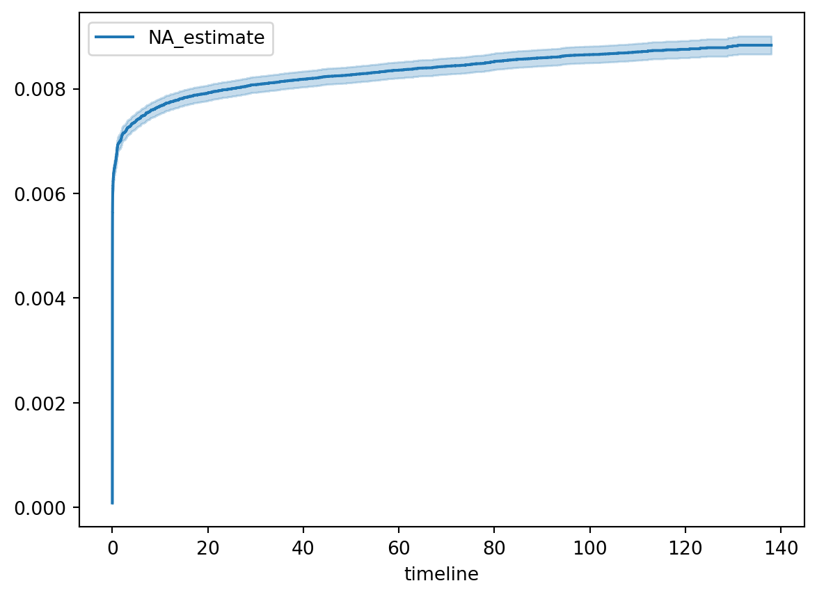
Let’s fit a cumulative hazard function to our data with the Lifelines package, probably the most popular Python survival analysis package. To keep things simple, we first convert our durations column from TimeDelta format to floating-point days. The notnull method of a Pandas series gives us a boolean flag that indicates if each unit has an observed endpoint or has a censored duration.
Code
durations["endpoint_observed"] = durations["endpoint"].notnull()durations["duration_days"] = ( durations["duration"].dt.total_seconds() / (60*60*24) # denom is number of seconds in a day)import lifelinesmodel = lifelines.NelsonAalenFitter()model.fit(durations["duration_days"], durations["endpoint_observed"])model.plot()
<AxesSubplot: xlabel='timeline'>
Example 2
Or, we could use the Scikit-survival package to fit a nonparametric survival curve.
Let’s plot the result, to confirm that something meaningful has happened. For our demo use case, it’s more natural to think of the conversion rate, which is just 1 minus the survival function.4
In upcoming articles, I’ll show how to convert other types of raw data into duration tables and how to interpret survival analysis results. Stay tuned! In the meantime, please leave a comment or question below. You can also contact me privately, with the Crosstab Kite contact form.
The Lifelines API documentation says that a duration matrix need not include all units, presumably omitting those with no observed endpoint. My concept of a duration table is different in that it should contain one row for each unit.↩︎
An exhaustive literature search is beyond the scope of this article, but here are some examples of works that avoid naming the input to survival models.
The R package survival uses the class Surv to define a “survival object” target variable, with both the duration and censoring indicator. The survfit.formula function has a data parameter but defines it only by saying it’s a data frame that includes the variables named in the Surv object.
Frank Harrell’s Regression Modeling Strategies does not appear to use an explicit term for the duration table. The survival analysis examples use datasets already in duration table format, named for their subject matter (e.g. prostate, p. 521)
The first step in preparation for [Kaplan-Meier] analysis involves the construction of a table…containing the three key elements required for input…The table is then sorted…Once this initial table is constructed…
Even the Lifelines package, from which I get the term duration matrix, is not consistent. It also uses the terms survival events and survival data for this concept.
Naming is hard and the field of survival analysis seems especially bad at it. I have more to say about this in a future post, but in the meantime, if you know of an existing, widespread, standard name for what I call duration table, please let me know.↩︎
Conversion data can also be left- or interval-censored. This article is only about right-censored data.↩︎
Technically, this is the cumulative incidence function.↩︎
Source Code
---title: "How to convert event logs to duration tables for survival analysis"author: "Brian Kent"date: "2021-06-07"image: tsvetoslav-hristov-QW-f6s9nFIs-unsplash.jpgcategories: [Python, survival analysis]description: | Survival models describe how much time it takes for some event to occur. This is a natural way to think about many applications but setting up the data can be tricky. In this article, we use Python to turn an event log into a duration table, which is the input format for many survival analysis tools.code-tools: trueformat: html: include-in-header: text: <link rel="canonical" href="https://www.crosstab.io/articles/events-to-durations/">---::: {.callout-tip}See also our article on creating duration tables from event logs in [SQL][sql-article].:::In many applications, it is most natural to think about how much time it takes for someoutcome to occur. In medicine, for example, we might ask whether a given treatmentincreases patients' life span. For predictive maintenance, we want to know which piecesof hardware have the shortest time until failure. For customer care, how long untilsupport tickets are resolved?**Survival analysis** techniques directly address these kinds of questions, but my senseis that survival modeling is relatively rare in industry data science. One reason mightbe that setting up the data for survival modeling can be tricky but most survivalanalysis literature skips the data prep part. I'll try to fill the gap, by showing howto create a **duration table** from an **event log**, using the example of web browserevents.## What is an event log?Event logs are a type of [transactional fact table][wiki-fact-table]. They have a[long-form][wiki-long-data] schema where each entry represents an event, defined by theunit (e.g. user), timestamp, and type of event.[Mixpanel's documentation][mixpanel-demo] shows an example log of user actions in a webbrowser. The key columns are `USERID` (the unit of interest), `TIMESTAMP`, and `EVENT`.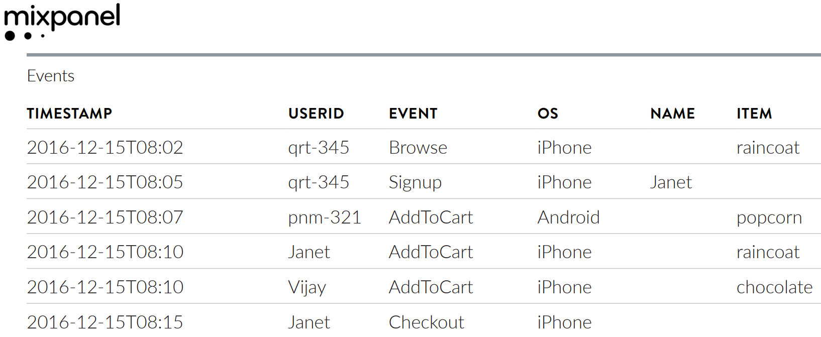For event logs, the event is a categorical variable. Contrast this with sensor output,which is typically numeric.## What's a duration table?A **duration table** is a wide-form table that shows for each unit whether the event ofinterest occurred, and if so, how long it took to happen. It is a common input dataformat for survival analysis software.A side note: the term *duration table* is based on the Python *Lifelines* package's term[duration matrix][lifelines-duration-matrix].^[The Lifelines API documentation says that a duration matrix need not include all units, presumably omitting those with no observed endpoint. My concept of a duration table is different in that it should contain one row for each unit.] Most of the literature I have read assumes we have this kind of data in hand and doesn't bother to give it an explicit name.[^duration-names][^duration-names]: An exhaustive literature search is beyond the scope of this article, but here are some examples of works that avoid naming the input to survival models. - The [Wikipedia entry for survival analysis][wiki-survival] shows an example of a duration table but only refers to it generically as a “survival data set”. - The R package `survival` uses the class [`Surv`][r-surv] to define a “survival object” target variable, with both the duration and censoring indicator. The [`survfit.formula`][r-survfit] function has a `data` parameter but defines it only by saying it's a data frame that includes the variables named in the `Surv` object. - Frank Harrell's [Regression Modeling Strategies][rms] does not appear to use an explicit term for the duration table. The survival analysis examples use datasets already in duration table format, named for their subject matter (e.g. `prostate`, p. 521) - Rich, et al. [A practical guide to understanding Kaplan-Meier curves][rich-paper] explicitly describes survival inputs as a table but never gives that table a name. > The first step in preparation for [Kaplan-Meier] analysis involves the > construction of a table...containing the three key elements required for > input...The table is then sorted...Once this initial table is constructed... - Even the Lifelines package, from which I get the term *duration matrix*, is not consistent. It also uses the terms *survival events* and *survival data* for this concept. Naming is hard and the field of survival analysis seems especially bad at it. I have more to say about this in a future post, but in the meantime, if you know of an existing, widespread, standard name for what I call *duration table*, please let me know.With the Mixpanel example, suppose we define conversion to be the *Checkout* event. Thenthe first part of the duration table for that event log would be:| UserID | Entry time | Conversion time | Conversion event || --- | --- | --- | --- || qrt-345 | 2016-12-15T08:02 | NA | NA || pnm-321 | 2016-12-15T08:07 | NA | NA || Janet | 2016-12-15T08:10 | 2016-12-15T08:15 | Checkout || Vijay | 2016-12-15T08:10 | NA | NA |The first two columns are straightforward. Each row corresponds to a user, indicated bythe user ID column. Entry time is the first recorded timestamp for each user.The missing values in the *Conversion time* and *Conversion event* columns are wherethings get interesting. **Here's the core insight of survival analysis: those users maystill convert in the future; we only know that they had not *yet* converted when theevent log was closed.** This is called [censoring][wiki-censoring] and it's somethingthat survival models handle gracefully, but we still need to represent it appropriatelyin our duration table.Suppose the Mixpanel log was closed at `2016-12-15T08:20`. The final duration table would be:| UserID | Entry time | Conversion time | Conversion event | Final observation time | Duration || --- | --- | --- | --- | --- | --- || qrt-345 | 2016-12-15T08:02 | NA | NA | 2016-12-15T08:20 | 18 seconds || pnm-321 | 2016-12-15T08:07 | NA | NA | 2016-12-15T08:20 | 13 seconds || Janet | 2016-12-15T08:10 | 2016-12-15T08:15 | Checkout | 2016-12-15T08:15 | 5 seconds || Vijay | 2016-12-15T08:10 | NA | NA | 2016-12-15T08:20 | 10 seconds |The *final observation time* is the conversion time if it's known or the timestamp ofthe last moment of observation (i.e. when the log was closed). The *duration* is thetime delta between the entry time and the final observation time. It will be our targetvariable in downstream modeling and is the field that is right-censored.^[Conversion data can also be left- or interval-censored. This article is only about right-censored data.]## The Metamorphosis### Input dataWe'll stick with the web browser example and use data from e-commerce site RetailRocket, [available on Kaggle][retailrocket-data]. The dataset has 2.8 million rows andoccupies about 250MB in memory.```{python}import pandas as pdevent_log = pd.read_csv("retailrocket_events.csv", dtype={"transactionid": "Int64"})event_log.index.name ="row"event_log["timestamp"] = pd.to_datetime(event_log["timestamp"], unit="ms")event_log.head()```### SchemaThe first thing we need to do is identify the schema of our event log. For **unit ofinterest**, let's go with *visitor* (`visitorid`), so we cananswer the questions *What fraction of users make a purchase and how long does it takethem to do so?* *Item* would also be an interesting unit of observation, and in real webbrowser data, we might also be interested in sessions.There are only three kinds of events: `view`, `addtocart`, and `transaction`:```{python}event_log["event"].value_counts()```The sequence of events for a visitor who completes a transaction looks like this:```{python}event_log.query("visitorid==1050575").sort_values("timestamp")```The visitor views a bunch of items, eventually adds a few to their cart, then purchasesthe items in the cart in a `transaction`. Let's define thetransaction event to be our **endpoint** of interest. Endpoints are the eventscorresponding to outcomes we're interested in; in clinical research, this might bedeath, disease recurrence, or recovery. In predictive maintenance, it could be hardwarefailure. In customer lifetime value, it would be reaching a revenue threshold. Inprinciple, we could have multiple endpoints, so we specify this in a list.Our schema is:```{python}unit ="visitorid"timestamp ="timestamp"event ="event"endpoints = ["transaction"]```### Find the entry time for each unitThe DataFrame `groupby` method is our workhorse because weneed to treat each visitor separately. The simplest way to define entry time for eachvisitor is to take the earliest logged timestamp:```{python}grp = event_log.groupby(unit)durations = pd.DataFrame(grp[timestamp].min())durations.rename(columns={timestamp: "entry_time"}, inplace=True)durations.head()```### Find each unit's endpoint time, if it existsFinding the endpoint time for each visitor is trickier because some visitors have notyet completed a transaction but might in the future. Furthermore, some users havecompleted multiple transactions, in which case we want the timestamp of the *earliest*endpoint event. We first filter the raw data down to just the endpoint events:```{python}endpoint_events = event_log.loc[event_log[event].isin(endpoints)]```then find the index (in the original DataFrame) of the earliest endpoint event for eachvisitor and extract just those rows. Remember that only the visitors who have anobserved endpoint are represented in the `endpoint_events`DataFrame.```{python}grp = endpoint_events.groupby(unit)idx_endpoint_events = grp[timestamp].idxmin() # these are indices in the original DataFrameendpoint_events = event_log.iloc[idx_endpoint_events].set_index(unit)endpoint_events.head()```Because Pandas DataFrames have well-crafted indexing, we can merge the endpoints andendpoint times back into our primary output table with simple column assignments. Ifyou're translating this to another language, be very careful about indexinghere---remember that these columns are not defined for every user.```{python}durations["endpoint"] = endpoint_events[event]durations["endpoint_time"] = endpoint_events[timestamp]durations.head()```### Compute the target variableOur target variable is the time it took for each unit to reach an endpoint *or* the**censoring time**, which is the end of our observation period. In the Mixpanel exampleabove we chose an arbitrary timestamp, but in practice it's usually easier to choose thecurrent time (e.g. `import datetime as dt; dt.datetime.now()`)or the latest timestamp in the log.We don't want to lose track of which users have an observed endpoint, so we'll createanother column that defaults to the censoring time unless a visitor has an endpointevent.```{python}censoring_time = event_log["timestamp"].max()durations["final_obs_time"] = durations["endpoint_time"].copy()durations["final_obs_time"].fillna(censoring_time, inplace=True)```The last step is to compute the elapsed time between each visitor's entry into thesystem and their final observed time. Once again Pandas makes this easy, returning a`TimeDelta`-type column by subtracting two timestamps.```{python}durations["duration"] = durations["final_obs_time"] - durations["entry_time"]durations.head()```Each row of the `durations` DataFrame represents a visitor.Each unit has an entry time, a final observation time, and the duration between thosetwo timestamps. We know whether or not a unit has reached an endpoint based on the `endpoint` and `endpoint_time` columns.### Sanity checksWe can sanity check the output using a few simple properties that should always be true,regardless of the input data. To start, we know that there should be one row in theoutput duration table for every unique `visitorid` in theevent log.```{python}assertlen(durations) == event_log[unit].nunique()```We can bound the `duration` variable by virtue of the way weconstructed it: using the earliest observation in the data for each visitor's entry timeand the latest timestamp overall as the censoring time.```{python}assert durations["duration"].max() <= ( event_log[timestamp].max() - event_log[timestamp].min())```And finally, we know that the number of visitors who have converted so far must be nobigger than the total number of endpoint events in the input log.```{python}assert ( durations["endpoint_time"].notnull().sum() <= event_log[event].isin(endpoints).sum())```## Next stepsNow we should be able to use any survival analysis software, with minimal additionaltweaks.### Example 1Let's fit a cumulative hazard function to our data with the [Lifelines][lifelines]package, probably the most popular Python survival analysis package. To keep thingssimple, we first convert our `durations` column from `TimeDelta`format to floating-point days. The `notnull` method of aPandas series gives us a boolean flag that indicates if each unit has an observedendpoint or has a censored duration.```{python}durations["endpoint_observed"] = durations["endpoint"].notnull()durations["duration_days"] = ( durations["duration"].dt.total_seconds() / (60*60*24) # denom is number of seconds in a day)import lifelinesmodel = lifelines.NelsonAalenFitter()model.fit(durations["duration_days"], durations["endpoint_observed"])model.plot()```### Example 2Or, we could use the [Scikit-survival][sksurv] package to fit a nonparametric survivalcurve.```{python}from sksurv.util import Survfrom sksurv.nonparametric import SurvivalFunctionEstimatortarget = Surv().from_dataframe("endpoint_observed", "duration_days", durations)model = SurvivalFunctionEstimator()model.fit(target)model.predict_proba([0, 20, 40, 60, 80, 100, 120])```Let's plot the result, to confirm that something meaningful has happened. For our demouse case, it's more natural to think of the conversion rate, which is just 1 minus thesurvival function.^[Technically, this is the **cumulative incidence function**.]```{python}import numpy as npimport plotly.express as pxtime_grid = np.linspace(0, 120, 1000)proba_survival = model.predict_proba(time_grid)conversion_rate =1- proba_survivalfig = px.line(x=time_grid, y=conversion_rate *100, template="plotly_white")fig.update_traces(line=dict(width=7))fig.update_layout(xaxis_title="Days elapsed", yaxis_title="Conversion rate (%)")fig.show()```In upcoming articles, I'll show how to convert other types of raw data into durationtables and how to interpret survival analysis results. Stay tuned! In the meantime,please leave a comment or question below. You can also contact me privately, with theCrosstab Kite [contact form][contact-page].## References* Listing image by Tsvetoslav Hristov on [Unsplash](https://unsplash.com/photos/QW-f6s9nFIs).[orig-article]: https://www.crosstab.io/articles/conversion-rate-model-tradeoffs[mixpanel-demo]: https://mixpanel.com/wp-content/uploads/2018/06/System-architecture_June2018.pdf[retailrocket-data]: https://www.kaggle.com/retailrocket/ecommerce-dataset?select=events.csv[wiki-long-data]: https://en.wikipedia.org/wiki/Wide_and_narrow_data[wiki-fact-table]: https://en.wikipedia.org/wiki/Fact_table[wiki-censoring]: https://en.wikipedia.org/wiki/Censoring_(statistics)[lifelines]: https://lifelines.readthedocs.io/en/latest/[lifelines-duration-matrix]: https://lifelines.readthedocs.io/en/latest/lifelines.utils.html#lifelines.utils.covariates_from_event_matrix[convoys]: https://better.engineering/convoys/[contact-page]: https://crosstab.webflow.io/contact[gist-code]: https://github.com/CrosstabKite/gists/blob/main/events_to_durations.py[wiki-survival]: https://en.wikipedia.org/wiki/Survival_analysis[r-survfit]:https://www.rdocumentation.org/packages/survival/versions/3.2-11/topics/survfit.formula[r-surv]: https://www.rdocumentation.org/packages/survival/versions/3.2-11/topics/Surv[rms]: https://link.springer.com/book/10.1007%2F978-3-319-19425-7[rich-paper]: https://citeseerx.ist.psu.edu/viewdoc/download?doi=10.1.1.945.3550&rep=rep1&type=pdf[sksurv]: https://scikit-survival.readthedocs.io/en/latest/index.html[sql-article]: ../events-to-durations-sql