How to use PyTorch LSTMs for time series regression

Warning

Readers have reported the data used in this article is no longer available. I am not actively maintaining this work, however, so please treat it “as is”. On a related note, check out my new project at https://theapricot.io!

Many machine learning applications that I’ve come across lately are time series regression tasks, where I want to predict a target variable from several input time series.

• Measure or forecast cell density in a bioreactor. Measuring directly is painful but direct proxies are too noisy.

• Classify a financial transaction as fraudulent or not based on a customer’s transaction history.

• Forecast (and optimize) crop yield based on a network of water, sun, and nutrient sensors.

I wanted to try LSTM models with these kinds of problems but found it tough to get started. Most LSTM tutorials focus on natural language processing, to the point where it can seem like LSTMs only work with text data. Searching for “LSTM time series” does return some hits, but they’re…not great.

So here’s my attempt; this article shows how to use PyTorch LSTMs for regression with multiple input time series. In particular, I’ll show how to forecast a target time series but once you have the basic data and model structure down, it’s not hard to adapt LSTMs to other types of supervised learning. Here’s the game plan:

1. Load, visualize, and preprocess the data
2. Define PyTorch Dataset and DataLoader objects
3. Define an LSTM regression model
4. Train and evaluate the model

In the interest of brevity, I’m going to skip lots of things. Most obviously, what’s an LSTM? For that, I suggest starting with the PyTorch tutorials, Andrej Karpathy’s intro to RNNs, and Christopher Olah’s intro to LSTMs. More advanced readers might be wondering:

• I thought attention was all I need? What about Transformers?
• Why PyTorch instead of Tensorflow or JAX?
• Why not try multiple layers in your LSTM? Where’s the hyperparameter tuning? What about rolling test sets?

All good questions…for another article. In the meantime, please see our Github repo for a Jupyter notebook version of the code snippets below.

Goal

Our goal in this demo is to forecast air quality in Austin—specifically, 2.5-micron particulate matter (PM2.5)—from sensors around the state of Texas.

Why would we do this, when there are plenty of PM2.5 sensors in Austin? Maybe we don’t want to buy a sensor of our own but we have a friend who will let us borrow one for a few weeks to collect training data. Or maybe we need a stand-in for the official EPA sensors when they go offline, which seems to happen often.¹

Data

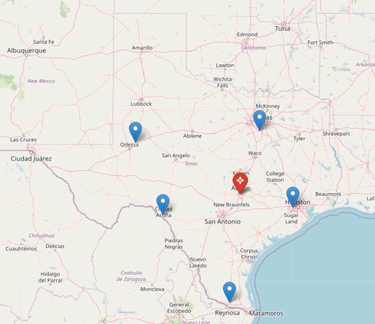
The data come from Purple Air, which sells sensors and makes (participating) customers’ data available for download. I downloaded seven weeks of this data from six sensors around the state of Texas.

Locations of the Purple Air sensors used in this article. We’ll create a model that forecasts the PM2.5 reading at the red sensor in Austin based on the data at the blue sensors around the rest of Texas.

For this demo, I’ve already preprocessed the data to align and sort the timestamps and interpolate a small number of missing values. Please see the preprocess_data.py script in the Github repo for the details. Let’s load the data and visualize it.²

Code

import pandas as pd

df = pd.read_csv("processed_pm25.csv", index_col="created_at")
print(df)

                           Del Rio  McAllen  Midlothian  Midland  Houston  \
created_at                                                                  
2021-09-01 00:00:00+00:00     5.37    23.39        4.79     7.57     7.60   
2021-09-01 00:02:00+00:00     5.95    23.02        4.60     8.50     7.78   
2021-09-01 00:04:00+00:00     5.84    25.49        5.70     8.07     7.64   
2021-09-01 00:06:00+00:00     7.07    25.22        5.18     8.66     7.69   
2021-09-01 00:08:00+00:00     5.18    23.16        5.29     7.98     7.74   
...                            ...      ...         ...      ...      ...   
2021-10-21 23:50:00+00:00     8.31     2.58        9.18    12.62     7.80   
2021-10-21 23:52:00+00:00     8.84     3.02       10.34    11.37     7.05   
2021-10-21 23:54:00+00:00     8.57     2.37       10.28    11.82     6.93   
2021-10-21 23:56:00+00:00     7.96     3.07       10.37    11.07     6.82   
2021-10-21 23:58:00+00:00     7.72     2.88       10.31    12.08     7.22   

                           Austin  
created_at                         
2021-09-01 00:00:00+00:00    8.32  
2021-09-01 00:02:00+00:00    8.93  
2021-09-01 00:04:00+00:00   10.10  
2021-09-01 00:06:00+00:00    9.24  
2021-09-01 00:08:00+00:00    9.02  
...                           ...  
2021-10-21 23:50:00+00:00   13.14  
2021-10-21 23:52:00+00:00   12.47  
2021-10-21 23:54:00+00:00   12.34  
2021-10-21 23:56:00+00:00   12.26  
2021-10-21 23:58:00+00:00   12.04  

[36720 rows x 6 columns]

The columns represent sensors and rows represent (sorted) timestamps. The values are PM2.5 readings, measured in micrograms per cubic meter.³

Plotting all six time series together doesn’t reveal much because there are a small number of short but huge spikes. The second plot is zoomed in to a y-axis range of [0, 60]; it shows clear long-run correlations between the sensors but lots of short-run variation both between and within the series. In other words, an interesting dataset!

Pardon a bit of Plotly styling boilerplate up front.

Code

import plotly.express as px
import plotly.graph_objects as go
import plotly.io as pio
pio.templates.default = "plotly_white"

plot_template = dict(
    layout=go.Layout({
        "font_size": 18,
        "xaxis_title_font_size": 24,
        "yaxis_title_font_size": 24})
)

fig = px.line(df, labels=dict(
    created_at="Date", value="PM2.5 (ug/m3)", variable="Sensor"
))
fig.update_layout(
  template=plot_template, legend=dict(orientation='h', y=1.02, title_text="")
)
fig.show()

Code

fig.update_yaxes(range = [0, 60])
fig.show()

Create the target variable

For our forecasting target, we need to shift the Austin sensor’s column forward in time. Let’s forecast 30 minutes in the future, which is 15 two-minute periods. The newly created target column won’t have values in the final 15 rows, so we’ll drop those.

Code

target_sensor = "Austin"
features = list(df.columns.difference([target_sensor]))

forecast_lead = 15
target = f"{target_sensor}_lead{forecast_lead}"

df[target] = df[target_sensor].shift(-forecast_lead)
df = df.iloc[:-forecast_lead]

Create a hold-out test set and preprocess the data

As always, we need a test set to evaluate our model. Here, we’ll keep it simple with a single temporal split, i.e. our test set is the last 11 days of data (about 23% of the total). The Scikit-learn user guide has a good discussion of temporal vs. random splits, if this is unfamiliar territory.

Code

test_start = "2021-10-10"

df_train = df.loc[:test_start].copy()
df_test = df.loc[test_start:].copy()

print("Test set fraction:", len(df_test) / len(df))

Test set fraction: 0.23498161013485902

Standardize the features and target

In my experience, standardizing both the features and the target seems to help substantially. This can also be done with Scikit-learn, but it’s really not that much code to do it with Python dictionaries and in this case, we really only need to keep the mean and standard deviation of the target column.

Code

target_mean = df_train[target].mean()
target_stdev = df_train[target].std()

for c in df_train.columns:
    mean = df_train[c].mean()
    stdev = df_train[c].std()

    df_train[c] = (df_train[c] - mean) / stdev
    df_test[c] = (df_test[c] - mean) / stdev

Create datasets that PyTorch DataLoader can work with

Important

If you’re skimming quickly, this is the part that really matters.

Typically, time series regression tutorials lessons show how to create features by extracting parts of the timestamps or by lagging features, that is, using past values of each feature as features in their own right. That’s not what we’re going to do with the LSTM; for each training instance, we’re going to give the model a sequence of observations.

One elegant way to do this is to create a PyTorch Dataset class, which is simpler than you might think. This strategy lets us lean on PyTorch’s nice DataLoader class to keep the model training and evaluation code super clean.

Our custom Dataset just needs to specify what happens when somebody requests the i’th element of the dataset. In a tabular dataset, this would be the i’th row of the table, but here we need to retrieve a sequence of rows.

So, given i and the sequence_length, we return the block of data from i - sequence_length through row i. If i is at the beginning of the dataset, we pad by repeating the first row as many times as needed to make the output have sequence_length rows. The only trick is avoiding off-by-1 errors in the slicing and padding.

All the magic happens in the __getitem__ method in this snippet.

Code

import torch
from torch.utils.data import Dataset

class SequenceDataset(Dataset):
    def __init__(self, dataframe, target, features, sequence_length=5):
        self.features = features
        self.target = target
        self.sequence_length = sequence_length
        self.y = torch.tensor(dataframe[target].values).float()
        self.X = torch.tensor(dataframe[features].values).float()

    def __len__(self):
        return self.X.shape[0]

    def __getitem__(self, i): 
        if i >= self.sequence_length - 1:
            i_start = i - self.sequence_length + 1
            x = self.X[i_start:(i + 1), :]
        else:
            padding = self.X[0].repeat(self.sequence_length - i - 1, 1)
            x = self.X[0:(i + 1), :]
            x = torch.cat((padding, x), 0)

        return x, self.y[i]

Let’s look at a small example to build intuition about how it works. Namely, let’s grab the 27’th entry in the dataset with a sequence length of 4.

Code

i = 27
sequence_length = 4

train_dataset = SequenceDataset(
    df_train,
    target=target,
    features=features,
    sequence_length=sequence_length
)

X, y = train_dataset[i]
print(X)

tensor([[-0.6169, -0.6339,  1.7142, -0.2673, -0.4447],
        [-0.7110, -0.5878,  1.7398, -0.5040, -0.3920],
        [-0.6076, -0.6504,  1.4540, -0.4670, -0.6426],
        [-0.5212, -0.7055,  1.4973, -0.5217, -0.5373]])

Our output feature tensor has a column for each of the five input sensors, and a row for each of the four time steps in the sequence. The last row is row 27 of the original table.

If we take index 28 instead, we see the rows are shifted forward in time by 1 step. The oldest row is popped off the back and row 28 is pushed onto the front.

Code

X, y = train_dataset[i + 1]
print(X)

tensor([[-0.7110, -0.5878,  1.7398, -0.5040, -0.3920],
        [-0.6076, -0.6504,  1.4540, -0.4670, -0.6426],
        [-0.5212, -0.7055,  1.4973, -0.5217, -0.5373],
        [-0.6385, -0.7607,  1.8232, -0.4331, -0.7225]])

Just to confirm, here’s the same logic for item 27, with Pandas DataFrame slicing.

Code

print(df_train[features].iloc[(i - sequence_length + 1): (i + 1)])

                            Del Rio   Houston   McAllen   Midland  Midlothian
created_at                                                                   
2021-09-01 00:48:00+00:00 -0.616850 -0.633936  1.714209 -0.267292   -0.444691
2021-09-01 00:50:00+00:00 -0.710992 -0.587842  1.739789 -0.503986   -0.392029
2021-09-01 00:52:00+00:00 -0.607590 -0.650398  1.453961 -0.466952   -0.642628
2021-09-01 00:54:00+00:00 -0.521165 -0.705546  1.497336 -0.521698   -0.537304

The next step is to set the dataset in a PyTorch DataLoader, which will draw minibatches of data for us. Let’s try a small batch size of 3, to illustrate. The feature tensor returned by a call to our train_loader has shape 3 x 4 x 5, which reflects our data structure choices:

• 3: batch size
• 4: sequence length
• 5: number of features

Code

from torch.utils.data import DataLoader
torch.manual_seed(99)

train_loader = DataLoader(train_dataset, batch_size=3, shuffle=True)

X, y = next(iter(train_loader))
print(X.shape)
print(X)

torch.Size([3, 4, 5])
tensor([[[ 0.2397, -0.2125, -0.0419,  0.1449, -0.1741],
         [ 0.2181, -0.1192, -0.0297,  0.0596, -0.3176],
         [ 0.3493, -0.2169, -0.1364,  0.1095, -0.1614],
         [-0.0505, -0.2811, -0.1965,  0.1803, -0.2885]],

        [[-1.1369, -0.5560, -1.1697, -1.2398, -1.1584],
         [-1.0876, -0.5758, -1.1463, -1.3107, -1.1638],
         [-1.0536, -0.7075, -1.1752, -1.1819, -1.1093],
         [-1.0675, -0.4946, -1.0540, -1.1271, -1.2255]],

        [[ 0.0622,  0.1738,  0.1572, -0.4734,  0.3434],
         [-0.0690,  0.1211,  0.4452, -0.5668,  0.3325],
         [-0.0165,  0.1464,  0.1594, -0.6086,  0.4760],
         [ 0.0159,  0.1859,  0.2595, -0.5716,  0.0111]]])

Create the datasets and data loaders for real

Now let’s do it for real, with a sequence of 30 time steps (60 minutes). For training, we’ll shuffle the data (the rows within each data sequence are not shuffled, only the order in which we draw the blocks). For the test set, shuffling isn’t necessary.

Code

torch.manual_seed(101)

batch_size = 4
sequence_length = 30

train_dataset = SequenceDataset(
    df_train,
    target=target,
    features=features,
    sequence_length=sequence_length
)
test_dataset = SequenceDataset(
    df_test,
    target=target,
    features=features,
    sequence_length=sequence_length
)

train_loader = DataLoader(train_dataset, batch_size=batch_size, shuffle=True)
test_loader = DataLoader(test_dataset, batch_size=batch_size, shuffle=False)

X, y = next(iter(train_loader))

print("Features shape:", X.shape)
print("Target shape:", y.shape)

Features shape: torch.Size([4, 30, 5])
Target shape: torch.Size([4])

The model and learning algorithm

With the hard data structure part done, now it’s all downhill from here! A few notes to highlight in the ShallowRegressionLSTM model below:

• Most importantly, we have to keep track of which dimension represents the batch in our input tensors. As we just saw, our data loaders use the first dimension for this, but the PyTorch LSTM layer’s default is to use the second dimension instead. So we set batch_first=True to make the dimensions line up, but confusingly, this doesn’t apply to the hidden and cell state tensors. In the forward method, we initialize h0 and c0 with batch size as the second dimension.

• We’ll hard code a single layer just to keep things simple.

• The output layer of the model is linear with a single output unit because we’re doing regression. This is one of only two lines of code that would need to change for a classification task.

Code

from torch import nn

class ShallowRegressionLSTM(nn.Module):
    def __init__(self, num_sensors, hidden_units):
        super().__init__()
        self.num_sensors = num_sensors  # this is the number of features
        self.hidden_units = hidden_units
        self.num_layers = 1

        self.lstm = nn.LSTM(
            input_size=num_sensors,
            hidden_size=hidden_units,
            batch_first=True,
            num_layers=self.num_layers
        )

        self.linear = nn.Linear(in_features=self.hidden_units, out_features=1)

    def forward(self, x):
        batch_size = x.shape[0]
        h0 = torch.zeros(self.num_layers, batch_size, self.hidden_units).requires_grad_()
        c0 = torch.zeros(self.num_layers, batch_size, self.hidden_units).requires_grad_()
        
        _, (hn, _) = self.lstm(x, (h0, c0))
        out = self.linear(hn[0]).flatten()  # First dim of Hn is num_layers, which is set to 1 above.

        return out

The other thing that would need to change is the loss function. Here we use the standard regression objective of mean square error, i.e. MSELoss.

I’ve chosen the learning rate and the number of hidden units by hand to get decent results with a model that trains relatively quickly on my laptop, but these would be great hyperparameters to experiment with more systematically.

Code

learning_rate = 5e-5
num_hidden_units = 16

model = ShallowRegressionLSTM(num_sensors=len(features), hidden_units=num_hidden_units)
loss_function = nn.MSELoss()
optimizer = torch.optim.Adam(model.parameters(), lr=learning_rate)

Training

Time to get the ship underway! The train_model and test_model functions below are standard PyTorch boilerplate; there is nothing in them specific to LSTMs or time series data. But that’s the point: by using a custom PyTorch Dataset and a DataLoader, we can use off-the-shelf training and evaluation loops.

Code

def train_model(data_loader, model, loss_function, optimizer):
    num_batches = len(data_loader)
    total_loss = 0
    model.train()
    
    for X, y in data_loader:
        output = model(X)
        loss = loss_function(output, y)

        optimizer.zero_grad()
        loss.backward()
        optimizer.step()

        total_loss += loss.item()

    avg_loss = total_loss / num_batches
    print(f"Train loss: {avg_loss}")

def test_model(data_loader, model, loss_function):
    
    num_batches = len(data_loader)
    total_loss = 0

    model.eval()
    with torch.no_grad():
        for X, y in data_loader:
            output = model(X)
            total_loss += loss_function(output, y).item()

    avg_loss = total_loss / num_batches
    print(f"Test loss: {avg_loss}")


print("Untrained test\n--------")
test_model(test_loader, model, loss_function)
print()

for ix_epoch in range(2):
    print(f"Epoch {ix_epoch}\n---------")
    train_model(train_loader, model, loss_function, optimizer=optimizer)
    test_model(test_loader, model, loss_function)
    print()

Untrained test
--------

Test loss: 1.0768692994880853

Epoch 0
---------

Train loss: 0.49809492697801305

Test loss: 0.6040830491229857

Epoch 1
---------

Train loss: 0.34119535735615947

Test loss: 0.6264536608196818

After just two epochs our test loss is already starting to climb, so it’s a good time to stop.

Evaluation

Evaluating the model is straightforward. First, let’s define a variant of the test function that actually returns the predictions. We also need a new DataLoader for the training set that isn’t shuffled, we can visualize the training and test set predictions chronologically. Lastly, it’s nice to un-standardize the predictions so they’re back in their original units of micrograms per cubic meter.

Code

def predict(data_loader, model):

    output = torch.tensor([])
    model.eval()
    with torch.no_grad():
        for X, _ in data_loader:
            y_star = model(X)
            output = torch.cat((output, y_star), 0)
    
    return output


train_eval_loader = DataLoader(train_dataset, batch_size=batch_size, shuffle=False)

ystar_col = "Model forecast"
df_train[ystar_col] = predict(train_eval_loader, model).numpy()
df_test[ystar_col] = predict(test_loader, model).numpy()

df_out = pd.concat((df_train, df_test))[[target, ystar_col]]

for c in df_out.columns:
    df_out[c] = df_out[c] * target_stdev + target_mean

print(df_out)

                           Austin_lead15  Model forecast
created_at                                              
2021-09-01 00:00:00+00:00           7.80        5.728048
2021-09-01 00:02:00+00:00           7.74        5.819161
2021-09-01 00:04:00+00:00           8.69        5.921119
2021-09-01 00:06:00+00:00           7.91        6.156377
2021-09-01 00:08:00+00:00           9.10        6.114249
...                                  ...             ...
2021-10-21 23:20:00+00:00          13.14        8.599350
2021-10-21 23:22:00+00:00          12.47        8.512151
2021-10-21 23:24:00+00:00          12.34        8.486712
2021-10-21 23:26:00+00:00          12.26        8.690888
2021-10-21 23:28:00+00:00          12.04        8.838891

[36705 rows x 2 columns]

Our purpose here isn’t a thorough investigation of model performance. The point—which we can see in the next plot—is that the model (red series) has learned something. On the test set (blue, starting October 10), the model fails to predict both the intra-hour squiggles and the big spikes, but successfully forecasts the “medium frequencies” It’s a start!

Code

fig = px.line(df_out, labels=dict(created_at="Date", value="PM2.5 (ug/m3)"))
fig.add_vline(x=test_start, line_width=4, line_dash="dash")
fig.add_annotation(xref="paper", x=0.75, yref="paper", y=0.8, text="Test set start", showarrow=False)
fig.update_layout(
    template=plot_template, legend=dict(orientation='h', y=1.02, title_text="")
)
fig.show()

Wrapping up

Hopefully, this walk-through has given you a sense for how to set up a time series regression problem using PyTorch LSTMs. Now the real work begins: experimenting with features, model families, architectures, and hyperparameters to get a result that’s good enough to deploy.

As always, please post comments, suggestions, and questions below or send me an email via the Contact page. Happy modeling!

Footnotes

1. Case in point: as I write this, the EPA air quality data website says “AirData query and visualization tools are currently not available due to unscheduled maintenance.”

2. I’m using Python 3.8, Pandas 1.3.4, Pytorch 1.10, and Plotly 5.1, on Ubuntu 20.04, CPU only.

3. The more common way to report PM2.5 is the EPA’s Air Quality Index (AQI), which is a scaled version of the raw micrograms per cubic meter reading.